Generalized Linear Models have landed in scikit-learn

While scikit-learn already had some Generalized Linear Models (GLM) implemented, e.g. LogisticRegression, other losses than mean squared error and log-loss were missing. As the world is almost (surely) never normally distributed, regression tasks might benefit a lot from the new PoissonRegressor, GammaRegressor and TweedieRegressor estimators: using those GLMs for positive, skewed data is much more appropriate than ordinary least squares and might lead to more adequate models. Starting from scikit-learn 0.23, GLMs are officially supported by scikit-learn and intended to be (or hopefully) continuously improving. They were part of  the Consortium roadmap since the beginning of the adventure. Read more below and in the User Guide.

The world is not normally distributed

Like real life, real world data is most often far from normality. Still, data is often assumed, sometimes implicitly, to follow a Normal (or Gaussian) distribution. The two most important assumptions made when choosing a Normal distribution or squared error for regression tasks are¹:

1. The data is distributed symmetrically around the expectation. Hence, expectation and median are the same.
2. The variance of the data does not depend on the expectation.

On top, it is well known to be sensitive to outliers. Here, we want to point out that—potentially better— alternatives are available.

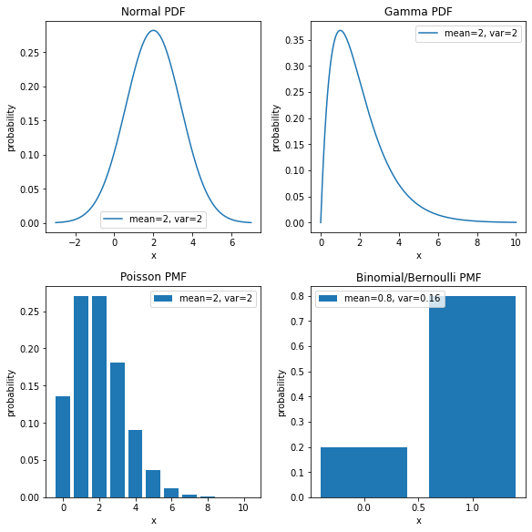
Typical instances of data that is not normally distributed are counts (discrete) or frequencies (counts per some unit). For these, the simple Poisson distribution might be much better suited. A few examples that come to mind are:

• number of clicks per second in a Geiger counter
• number of patients per day in a hospital
• number of persons per day using their bike
• number of goals scored per game and player
• number of smiles per day and person … Would love to have those data! Think about making their distribution more normal!

In what follows, we have chosen the diamonds dataset to show the non-normality and the convenience of GLMs in modelling such targets.

The diamonds dataset consists of prices of over 50 000 round cut diamonds with a few explaining variables, also called features X, such as ‘carat’, ‘color’, ‘cut quality’, ‘clarity’ and so forth. We start with a plot of the (marginal) cumulative distribution function (CDF) of the target variable price and compare to a fitted Normal and Gamma distribution which have both two parameters each.

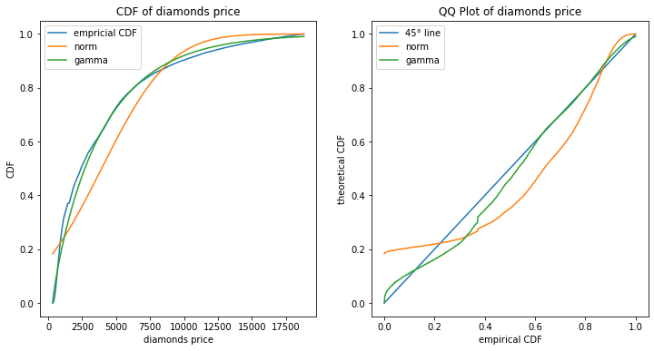
These plots show clearly that the Gamma distribution might be a better fit to the marginal distribution of Y than the Normal distribution.

Let’s start with a more theoretical intermezzo in the next section, we will resume to the diamonds dataset after.

Introduction to GLMs

GLMs in a Nutshell

GLMs are statistical models for regression tasks that aim to estimate and predict the conditional expectation of a target variable Y, i.e. E[Y|X]. They unify many different target types under one framework: Ordinary Least Squares, Logistic, Probit and multinomial model, Poisson regression, Gamma and many more. GLMs were formalized by John Nelder and Robert Wedderburn in 1972, long after artificial neural networks!

The basic assumptions for an instance or data row i are

• E[Y_i|x_i] = μ_i= h(x_i · β),
• Var[Y_i|x_i] ∼ v(μ_i) / w_i,

where μ_i is the mean of the conditional distribution of Y given x_i.

One needs to specify:

1. the target variable Y_i,
2. the inverse link function h, which maps real numbers to the range of Y (or more precisely the range of E[Y]),
3. optionally, sample weights w_i,
4. the variance function v(μ), which is equivalent to specifying a loss function or a specific distribution from the family of the exponential dispersion model (EDM),
5. the feature matrix X with row vectors x_i,
6. the coefficients or weights beta to be estimated from the data.

Note that the choice of the loss or distribution function or, equivalently, the variance function is crucial. It should, at least, reflect the domain of Y.

Some typical examples combinations are:

1. measurement errors are described as real numbers, with a Normal distribution and an identity link function;
2. insurance claims are represented by positive numbers, with a Gamma distribution and a log link function;
3. Geiger counts are non-negative numbers, with a Poisson distribution and a log link function;
4. the probability of success of a challenge are numbers in the [0, 1] interval, with a Binomial distribution and a logit link function

Once you have chosen the first four points, what remains to do is to find a good feature matrix X. Unlike other machine learning algorithms such as boosted trees, there are very few hyperparameters to tune. A typical hyperparameter is the regularization strength when penalties are applied. Therefore, the biggest leverage to improve your GLM is manual feature engineering of X. This includes, among others, feature selection, encoding schemes for categorical features, interaction terms, non-linear terms like x².

Strengths

• Very well understood and established, proven over and over in practice, e.g. stability, see next point.
• Very stable: slight changes of training data do not alter the fitted model much (counter example: decision trees).
• Versatile as to model different targets with different link and loss functions.
  As an example, Log link gives a multiplicative structure and effects are interpreted on a relative scale.
  Together with a Poisson distribution, this still works even when some target values are exactly zero.
• Mathematical tractable which means a good theoretical understanding and a fast fitting even for large datasets.
• Ease of interpretation.
• As flexible as the building of the feature matrix X.
• Some losses, like Poisson loss, can handle a certain amount of excess of zeros.

Weaknesses

• Feature matrix X has to be built manually, in particular interaction terms and non-linear effects.
• Unbiaseness depends on (correct) specification of X and on combination of link and loss function.
• Predictive performance often worse than for boosted tree models or neural networks.

Current Minimal Implementation in Scikit-Learn

The new GLM regressors are available as
from sklearn.linear_model import PoissonRegressor
from sklearn.linear_model import GammaRegressor
from sklearn.linear_model import TweedieRegressor

The TweedieRegressor has a parameter power, which corresponds to the exponent of the variance function v(μ) ∼ μ^p. For ease of the most common use, PoissonRegressor and GammaRegressor are the same as TweedieRegressor(power=1) and TweedieRegressor(power=2), respectively, with built-in log link. All of them also support an L2-penalty on the coefficients by setting the penalization strength alpha. The underlying optimization problem is solved via the l-bfgs solver of scipy. Note that the scikit-learn release 0.23 also introduced the Poisson loss for the histogram gradient boosting regressor as HistGradientBoostingRegressor(loss='poisson').

Gamma GLM for Diamonds

After all this theory, it is time to come back to our real world dataset: diamonds.
Although, in the first section, we were analysing the marginal distribution of Y and not the conditional (on the features X) distribution, we take the plot as a hint to fit a Gamma GLM with log-link, i.e. h(x) = exp(x). Furthermore, we split the data textbook-like into 80% training set and 20% test set² and use ColumnTransformer to handle columns differently. Our feature engineering consists of selecting only the four columns ‘carat’, ‘clarity’, ‘color’ and ‘cut’, log-transforming ‘carat’ as well as one-hot-encoding the other three. Fitting a Gamma distribution and predicting on the test sample gives us the plot below.

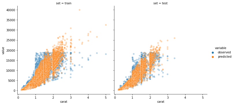
Note that fitting Ordinary Least Squares on log(‘price’) works also quite well. This is to be expected, as Log-Normal and Gamma are very similar distributions, both with Var[Y] ∼ E[Y]² = μ².

Outlook

There are several open issues and pull requests for improving GLMs and fitting of non-normal data. Some of them have been implemented in scikit-learn 0.24 already, let’s hope the others will be merged in the near future:

• Poisson splitting criterion for decision trees (PR #17386) made it in v0.24.
• Spline Transformer (PR #18368) will be available in 1.0.
• L1 penalty and coordinate descent solver (Issue #16637),
• IRLS solver if benchmarks show improvement over l-bfgs (Issue #16634),
• Better support for interaction terms (Issue #15263),
• Native categorical support (Issue #18893),
• Feature names Enhancement Proposal (SLEP015) is under active discussion.

By Christian Lorentzen

Footnotes

¹ Algorithms and estimation methods are often well able to deal with some deviation from the Normal distribution. In addition, the central limit theorem justifies a Normal distribution when considering averages or means, and the Gauss–Markov theorem is a cornerstone for usage of least squares with linear estimators (linear in the target Y).

² Rows in the diamonds dataset seem to be highly correlated as there are many rows with the same values for carat, cut, color, clarity and price, while the values for x, y and z seem to be permuted.
Therefore, we define a new group variable that is unique for ‘carat’, ‘cut’, ‘color’, ‘clarity’ and ‘price’.
Then, we split stratified by group, i.e. using a GroupShuffleSplit.
Having correlated train and test sets invalidates the independent and identical distributed assumption and may render test scores too optimistical.